
Though I’m primarily settled on ggplot2 for static plots, I’m always on the lookout for techniques to make interactive visualizations. echarts4r is just one of my new favored deals for this. It’s intuitive, highly effective, and flexible.
The echarts4r package is an R wrapper for the echarts JavaScript library, an formal Apache Software package Foundation undertaking (it graduated from incubator standing in December). That can help me experience confident I can rely on the JavaScript code fundamental the R package.
So let’s get a seem at echarts4r.
Deal creator John Coene points out the essentials in a having started out website page:
- Every operate in the package starts off with
e_. - You commence coding a visualization by creating an echarts item with the
e_charts()operate. That will take your data frame and x-axis column as arguments. - Up coming, you insert a operate for the sort of chart (
e_line(),e_bar(), and so on.) with the y-axis sequence column identify as an argument. - The rest is primarily customization!
Let us get a seem.
Line charts with echarts4r
For example data, I downloaded and wrangled some housing price tag info by US city from Zillow. If you want to adhere to along, data instructions are at the end of this report.
My residences_wide data frame has just one column for Thirty day period (I’m just hunting at December for every yr commencing in 2007) and columns for every city.
Classes ‘data.table’ and 'data.frame':fourteen obs. of  10 variables:
 $ Thirty day period        : Variable w/ fourteen stages "2007-twelve-31","2008-twelve-31",..: 1 two three 4 five six seven eight nine 10 ...
 $ Austin       : num  247428 240695 237653 232146 230383 ...
 $ Boston       : num  400515 366284 352017 363261 353877 ...
 $ Charlotte    : num  193581 185012 174552 162368 150636 ...
 $ Chicago      : num  294717 254638 215646 193368 171936 ...
 $ Dallas       : num  142281 129887 130739 122384 115999 ...
 $ New York     : num  534711 494393 459175 461231 450736 ...
 $ Phoenix      : num  239798 177223 141344 123984 114166 ...
 $ San Francisco: num  920275 827897 763659 755145 709967 ...
 $ Tampa        : num  248325 191450 153456 136778 120058 ...
I’ll commence by loading the echarts4r and dplyr deals. Note I’m using the progress variation of echarts4r to access the hottest variation of the echarts JavaScript library. You can set up the dev variation with these strains:
fobs::set up_github"JohnCoene/echarts4r")
library(echarts4r)
library(dplyr)
In the code below, I make a simple echarts4r item with Thirty day period as the x-axis column.
residences_huge {36a394957233d72e39ae9c6059652940c987f134ee85c6741bc5f1e7246491e6}>{36a394957233d72e39ae9c6059652940c987f134ee85c6741bc5f1e7246491e6}
e_charts(x = Thirty day period)
If you are common with ggplot, this first step is similar: It creates an item, but there is no data in the visualization however. You’ll see the x axis but no y axis or data.
Relying on your browser width, all the axis labels could not display screen mainly because echarts4r is responsive by default — you never have to fret about the axis text labels overwriting every other if you can find not ample room for them all.
Up coming, I’ll insert the sort of chart I want and the y-axis column. For a line chart, that is the e_line() operate. It demands at least just one argument, the column with the values. The argument is called serie, as in singular of sequence.
residences_huge {36a394957233d72e39ae9c6059652940c987f134ee85c6741bc5f1e7246491e6}>{36a394957233d72e39ae9c6059652940c987f134ee85c6741bc5f1e7246491e6}
e_charts(x = Thirty day period) {36a394957233d72e39ae9c6059652940c987f134ee85c6741bc5f1e7246491e6}>{36a394957233d72e39ae9c6059652940c987f134ee85c6741bc5f1e7246491e6}
e_line(serie = `San Francisco`)
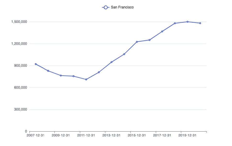 Display shot by Sharon Machlis, IDG
Line chart of Zillow data made with echarts4r.
There are lots of other chart varieties readily available, like bar charts with e_bar(), region charts e_region(), scatter plots e_scatter(), box plots e_boxplot(), histograms e_histogram(), warmth maps e_heatmap(), tree maps e_tree(), term clouds e_cloud(), and pie charts e_pie(). You can see the comprehensive listing on the echarts4r package site or in the enable documents.
Every of the chart-sort capabilities get column names with no quotation marks as arguments. That is similar to how ggplot operates.
But most capabilities mentioned here have versions that get quoted column names. That lets you use variable names as arguments. John Coene calls all those “escape-hatch” capabilities, and they have an underscore at the end of the operate identify, these kinds of as:
e_line(Boston)
my_city <- "Boston"
e_line_(my_city)
This would make it uncomplicated to make capabilities out of your chart code.
Up coming, I’ll insert a 2nd city with another e_line() operate.
residences_huge {36a394957233d72e39ae9c6059652940c987f134ee85c6741bc5f1e7246491e6}>{36a394957233d72e39ae9c6059652940c987f134ee85c6741bc5f1e7246491e6}
e_charts(x = Thirty day period) {36a394957233d72e39ae9c6059652940c987f134ee85c6741bc5f1e7246491e6}>{36a394957233d72e39ae9c6059652940c987f134ee85c6741bc5f1e7246491e6}
e_line(serie = `San Francisco`) {36a394957233d72e39ae9c6059652940c987f134ee85c6741bc5f1e7246491e6}>{36a394957233d72e39ae9c6059652940c987f134ee85c6741bc5f1e7246491e6}
e_line(serie = Boston)
There are no tooltips displayed by default, but I can insert all those with the e_tooltips() operate. Discover that commas are additional to the tooltip values by default, which is nice.
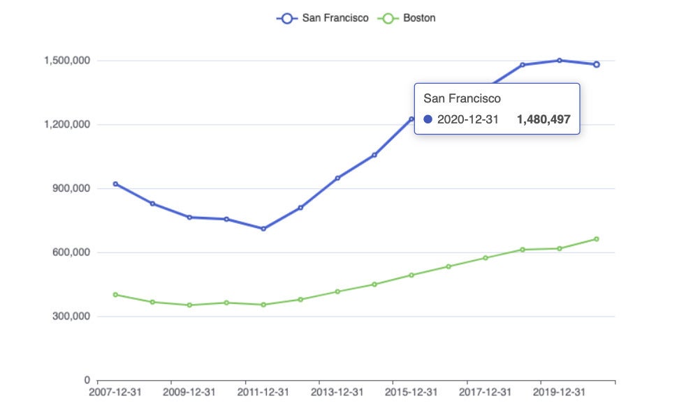 Display shot by Sharon Machlis, IDG
echarts4r line chart with two sequence and tooltips.
But the tooltip here could be even far more practical if I could see both equally values at the similar time. I can do that with this operate:
e_tooltip(set off = "axis")
I can turn this line chart into a grouped bar chart just by swapping in e_bar() for e_line().
Customize chart colors with echarts4r
You’ll most likely want to customise the colors for your charts at some stage. There are thirteen developed-in themes, which you can see on the echarts4r site. In the code below, I first conserve my chart in a variable referred to as p so I never have to maintain repeating that code. Then I add a theme, in this circumstance bee-encouraged, with e_theme("bee-encouraged")
p <- houses_wide {36a394957233d72e39ae9c6059652940c987f134ee85c6741bc5f1e7246491e6}>{36a394957233d72e39ae9c6059652940c987f134ee85c6741bc5f1e7246491e6}
e_charts(x = Thirty day period) {36a394957233d72e39ae9c6059652940c987f134ee85c6741bc5f1e7246491e6}>{36a394957233d72e39ae9c6059652940c987f134ee85c6741bc5f1e7246491e6}
e_line(serie = `San Francisco`) {36a394957233d72e39ae9c6059652940c987f134ee85c6741bc5f1e7246491e6}>{36a394957233d72e39ae9c6059652940c987f134ee85c6741bc5f1e7246491e6}
e_line(serie = Boston) {36a394957233d72e39ae9c6059652940c987f134ee85c6741bc5f1e7246491e6}>{36a394957233d72e39ae9c6059652940c987f134ee85c6741bc5f1e7246491e6}
e_tooltip(set off = "axis")
p {36a394957233d72e39ae9c6059652940c987f134ee85c6741bc5f1e7246491e6}>{36a394957233d72e39ae9c6059652940c987f134ee85c6741bc5f1e7246491e6}
e_theme("bee-encouraged")
You can make your own theme from scratch or modify an current just one. There is an on the net theme builder software to enable. To use that software, make your customizations, download the JSON file for your theme, and use e_theme_personalized("identify_of_my_theme") to insert it to a plot.
You can also tweak a theme proper in your graph code — for example, shifting a theme’s qualifications color with code these kinds of as:
p {36a394957233d72e39ae9c6059652940c987f134ee85c6741bc5f1e7246491e6}>{36a394957233d72e39ae9c6059652940c987f134ee85c6741bc5f1e7246491e6}
e_theme_personalized("mytheme.json") {36a394957233d72e39ae9c6059652940c987f134ee85c6741bc5f1e7246491e6}>{36a394957233d72e39ae9c6059652940c987f134ee85c6741bc5f1e7246491e6}
e_color(qualifications = "ivory")
You never will need to use a theme to customise your graph, even so the e_color() operate operates on graph defaults as nicely. The first argument for e_color() is a vector of colors for your strains, bars, factors, whatever. Beneath I first make a vector of a few colors (using color names or hex values). Then I insert that vector as the first argument to e_color():
my_colors <- c("darkblue", "#03925e", "purple")
p <- houses_wide {36a394957233d72e39ae9c6059652940c987f134ee85c6741bc5f1e7246491e6}>{36a394957233d72e39ae9c6059652940c987f134ee85c6741bc5f1e7246491e6}
e_charts(x = Thirty day period) {36a394957233d72e39ae9c6059652940c987f134ee85c6741bc5f1e7246491e6}>{36a394957233d72e39ae9c6059652940c987f134ee85c6741bc5f1e7246491e6}
e_line(serie = `San Francisco`) {36a394957233d72e39ae9c6059652940c987f134ee85c6741bc5f1e7246491e6}>{36a394957233d72e39ae9c6059652940c987f134ee85c6741bc5f1e7246491e6}
e_line(serie = Boston) {36a394957233d72e39ae9c6059652940c987f134ee85c6741bc5f1e7246491e6}>{36a394957233d72e39ae9c6059652940c987f134ee85c6741bc5f1e7246491e6}
e_line(serie = Austin) {36a394957233d72e39ae9c6059652940c987f134ee85c6741bc5f1e7246491e6}>{36a394957233d72e39ae9c6059652940c987f134ee85c6741bc5f1e7246491e6}
e_tooltip(set off = "axis") {36a394957233d72e39ae9c6059652940c987f134ee85c6741bc5f1e7246491e6}>{36a394957233d72e39ae9c6059652940c987f134ee85c6741bc5f1e7246491e6}
e_color(my_colors)
RColorBrewer palettes
I never see RColorBrewer palettes developed into echarts4r the way they are in ggplot, but it’s effortless to insert them yourself. In the subsequent code team, I load the RColorBrewer library and make a vector of colors with the brewer.pal() operate. I want a few colors using the Dark2 palette (just one of my favorites):
library(RColorBrewer)
my_colors <- brewer.pal(3, "Dark2")
my_colors
## [1] "#1B9E77" "#D95F02" "#7570B3"
p {36a394957233d72e39ae9c6059652940c987f134ee85c6741bc5f1e7246491e6}>{36a394957233d72e39ae9c6059652940c987f134ee85c6741bc5f1e7246491e6}
e_color(my_colors)
 Display shot by Sharon Machlis, IDG
echarts4r line chart with an RColorBrewer palette.
Paletteer palettes
By the way, a similar structure lets you use the R paletteer package to access a load of R palettes from lots of various R palette deals. The code below seems at the Colour_Blind palette from the ggthemes selection and selects the first, 2nd, and fifth of all those colors.
library(paletteer)
paletteer_d("ggthemes::Colour_Blind")
my_colors <- paletteer_d("ggthemes::Color_Blind")[c(1,2,5)]
p {36a394957233d72e39ae9c6059652940c987f134ee85c6741bc5f1e7246491e6}>{36a394957233d72e39ae9c6059652940c987f134ee85c6741bc5f1e7246491e6}
e_color(my_colors)
 Display shot by Sharon Machlis, IDG
Colour-blind palette from ggthemes
If you are not common with the paletteer package, the operate paletteer_d() accesses any of the readily available discreet color palettes. Listed here I wanted Color_Blind from ggthemes, and I selected colors 1, two, and five for the my_colors vector.
Lengthy-structure “tidy” data
If there are a good deal of sequence in your data, you most likely never want to sort out every just one by identify in a different operate phone. And you never have to. echarts4r handles prolonged-structure “tidy” data elegantly.
For this team of illustrations, I’ll use a data frame in prolonged structure with apartment price tag info. Information on how to make your own copy of the data is at the end of this report.
Do not miss out on the following code team: I use dplyr’s team_by() operate on the data frame prior to running e_charts() on it, and echarts4r understands that. Now if I convey to echarts4r to use Thirty day period for the x axis and Price for the y axis, it knows to plot every team as a different sequence. (I’m also preserving this graph to a variable referred to as myplot.)
myplot <- condos {36a394957233d72e39ae9c6059652940c987f134ee85c6741bc5f1e7246491e6}>{36a394957233d72e39ae9c6059652940c987f134ee85c6741bc5f1e7246491e6}
team_by(Town) {36a394957233d72e39ae9c6059652940c987f134ee85c6741bc5f1e7246491e6}>{36a394957233d72e39ae9c6059652940c987f134ee85c6741bc5f1e7246491e6} #<<
e_charts(x = Thirty day period) {36a394957233d72e39ae9c6059652940c987f134ee85c6741bc5f1e7246491e6}>{36a394957233d72e39ae9c6059652940c987f134ee85c6741bc5f1e7246491e6}
e_line(serie = Price) {36a394957233d72e39ae9c6059652940c987f134ee85c6741bc5f1e7246491e6}>{36a394957233d72e39ae9c6059652940c987f134ee85c6741bc5f1e7246491e6}
e_tooltip(set off = "axis")
myplot
 Display shot by Sharon Machlis, IDG
echarts4r line chart with legend at the major.
The legend at the major of the graph is not really practical, nevertheless. If I want to come across Tampa (the pink line), I can mouse in excess of the legend, but it will still be challenging to see the highlighted pink line with so lots of other strains proper in close proximity to it. The good thing is, you can find a resolution.
Custom made legend
In the following code team, I insert capabilities e_grid() and e_legend() to the graph.
myplot {36a394957233d72e39ae9c6059652940c987f134ee85c6741bc5f1e7246491e6}>{36a394957233d72e39ae9c6059652940c987f134ee85c6741bc5f1e7246491e6}
e_grid(proper = '15{36a394957233d72e39ae9c6059652940c987f134ee85c6741bc5f1e7246491e6}') {36a394957233d72e39ae9c6059652940c987f134ee85c6741bc5f1e7246491e6}>{36a394957233d72e39ae9c6059652940c987f134ee85c6741bc5f1e7246491e6}
e_legend(orient = 'vertical',
proper = '5', major = '15{36a394957233d72e39ae9c6059652940c987f134ee85c6741bc5f1e7246491e6}')
The e_grid(proper = '15{36a394957233d72e39ae9c6059652940c987f134ee85c6741bc5f1e7246491e6}') says I want my most important graph visualization to have 15{36a394957233d72e39ae9c6059652940c987f134ee85c6741bc5f1e7246491e6} padding on the proper aspect. The e_legend() operate says to make the legend vertical as an alternative of horizontal, insert a 5-pixel padding on the proper, and insert a 15{36a394957233d72e39ae9c6059652940c987f134ee85c6741bc5f1e7246491e6} padding on the major.
 Display shot by Sharon Machlis, IDG
Line chart with legend on the aspect.
That can help, but if I want to only see Tampa, I will need to click on each other legend merchandise to turn it off. Some interactive data visualization resources permit you double-click an merchandise to just present that just one. echarts handles this a tiny differently: You can insert buttons to “invert” the choice process, so you only see the merchandise you click.
To do this, I additional a selector argument to the e_legend() operate. I observed all those buttons in a sample echart JavaScript chart that employed selector, but (as significantly as I know) it’s not developed-in performance in echarts4r. John only challenging-coded some of the performance in the wrapper but we can use all of it — with the proper syntax.
Translate JavaScript into echarts4r R code
A swift detour for a tiny “how this operates under the hood” explanation. Beneath is an example John Coene has on the echarts4r internet site. You can see the original echarts JavaScript documentation in the graphic (you are going to most likely will need to click to broaden it): tooltip.axisPointer.sort. tooltip is an readily available echarts4r operate, e_tooltip(), so we can use that in R. axisPointer is a tooltip alternative, but it’s not element of the R package. One particular of axisPointer’s solutions is sort, which can have a benefit of line, shadow, none, or cross.
 Apache Software package Foundation
So, we will need to translate that JavaScript into R. We can do that by using axisPointer as an argument of e_tooltip(). Here’s the significant element: For the benefit of axisPointer, we make a listing, with the listing containing sort = "cross".
e_tooltip(axisPointer = listing(sort = "cross"))
If you know how this operates, you have all the electric power and flexibility of the overall echarts JavaScript library, not only the capabilities and arguments John Coene coded into the package.
To make two selector buttons, this is the JavaScript syntax from the echarts internet site:
selector: [

sort: 'inverse',
title: 'Invert'
,

sort: 'all or inverse',
title: 'Inverse'

]
And this is the R syntax:
e_legend(
selector = listing(
listing(sort = 'inverse', title = 'Invert'),
listing(sort = 'all', title = 'Reset')
)
)
Every essential-benefit pair gets its own listing within just the selector listing. Everything’s a listing, at times nested. That is it!
Plot titles in echarts4r
Alright let’s turn to a little something less complicated: a title for our graph. echarts4r has an e_title() operate that can get arguments text for the title text, subtext for the subtitle text, and also hyperlink and sublink if you want to insert a clickable URL to either the title or subtitle.
If I want to alter the alignment of the headline and subheadline, the argument is remaining. remaining can get a selection for how substantially padding you want involving the remaining edge and the commence of text, or it can get centre or proper for alignment as you see here:
myplot {36a394957233d72e39ae9c6059652940c987f134ee85c6741bc5f1e7246491e6}>{36a394957233d72e39ae9c6059652940c987f134ee85c6741bc5f1e7246491e6}
e_title(text = "Regular monthly Median Solitary-Spouse and children Residence Prices",
subtext = "Source: Zillow.com",
sublink = "https://www.zillow.com/investigate/data/",
remaining = "centre"
)
remaining = "centre" is not really intuitive for new customers, but it does make some feeling if you know the qualifications.
Colour charts by group with echarts4r
For these color-by-team demos, I’ll use a data set with columns for the city, thirty day period, apartment benefit, single-spouse and children household benefit, and “region” (which I just designed up for purposes of coloring by team it’s not a Zillow region).
head(all_data_w_sort_columns, two)
    Town      Thirty day period  Condominium SingleFamily Location
1 Austin 2007-twelve-31 221734       247428  South
two Austin 2008-twelve-31 210860       240695  South
Beneath is code for a scatter plot to see if single-spouse and children and apartment price ranges go in tandem. Mainly because I employed dplyr’s team_by() on the data prior to creating a scatter plot, the plot is colored by region. I was also in a position to set the dot dimension with image_dimension.
This code block adds a little something else to the plot: a couple of “toolbox features” at the major proper of the graph. I involved zoom, reset, look at the fundamental data, and conserve the plot as an graphic, but there are numerous other folks.
all_data_w_sort_columns {36a394957233d72e39ae9c6059652940c987f134ee85c6741bc5f1e7246491e6}>{36a394957233d72e39ae9c6059652940c987f134ee85c6741bc5f1e7246491e6}
team_by(Location) {36a394957233d72e39ae9c6059652940c987f134ee85c6741bc5f1e7246491e6}>{36a394957233d72e39ae9c6059652940c987f134ee85c6741bc5f1e7246491e6}
e_charts(SingleFamily) {36a394957233d72e39ae9c6059652940c987f134ee85c6741bc5f1e7246491e6}>{36a394957233d72e39ae9c6059652940c987f134ee85c6741bc5f1e7246491e6}
e_scatter(Condominium, image_dimension = six) {36a394957233d72e39ae9c6059652940c987f134ee85c6741bc5f1e7246491e6}>{36a394957233d72e39ae9c6059652940c987f134ee85c6741bc5f1e7246491e6}
e_legend(Bogus) {36a394957233d72e39ae9c6059652940c987f134ee85c6741bc5f1e7246491e6}>{36a394957233d72e39ae9c6059652940c987f134ee85c6741bc5f1e7246491e6}
e_tooltip() {36a394957233d72e39ae9c6059652940c987f134ee85c6741bc5f1e7246491e6}>{36a394957233d72e39ae9c6059652940c987f134ee85c6741bc5f1e7246491e6}
e_toolbox_element("dataZoom") {36a394957233d72e39ae9c6059652940c987f134ee85c6741bc5f1e7246491e6}>{36a394957233d72e39ae9c6059652940c987f134ee85c6741bc5f1e7246491e6}
e_toolbox_element(element = "reset") {36a394957233d72e39ae9c6059652940c987f134ee85c6741bc5f1e7246491e6}>{36a394957233d72e39ae9c6059652940c987f134ee85c6741bc5f1e7246491e6}
e_toolbox_element("dataView") {36a394957233d72e39ae9c6059652940c987f134ee85c6741bc5f1e7246491e6}>{36a394957233d72e39ae9c6059652940c987f134ee85c6741bc5f1e7246491e6}
e_toolbox_element("saveAsImage")
 Display shot by Sharon Machlis, IDG
There are numerous statistical capabilities readily available, like regression strains and error bars, these kinds of as e_lm(Condominium ~ SingleFamily, color = "eco-friendly") to insert a linear regression line.
Animations with echarts4r
I’ll wrap up our echarts4r tour with some effortless animations.
For these demos, I am going to use data from the US CDC on vaccinations by state: doses administered in comparison to vaccine doses obtained, to see which states are executing the best task of having vaccines they have into people’s arms speedily. The column I want to graph is PctUsed. I also additional a color column if I want to spotlight just one state with a various color, in this circumstance Massachusetts.
You can download the data from GitHub:
mydata <- readr::read_csv("https://gist.githubusercontent.com/smach/194d26539b0d0deb9f6ac5ca2e7d49d0/raw/f0d3362e06e3cb7dbfc0c9df67e259f1e9dfb898/timeline_data.csv")
str(mydata)
spec_tbl_df [112 × seven] (S3: spec_tbl_df/tbl_df/tbl/data.frame)
 $ State            : chr [1:112] "CT" "MA" "ME" "NH" ...
 $ TotalDistributed : num [1:112] 740300 1247600 254550 257700 3378300 ...
 $ TotalAdministered: num [1:112] 542414 806376 178449 166603 2418074 ...
 $ ReportDate       : Date[1:112], structure: "2021-02-08" "2021-02-08" "2021-02-08" "2021-02-08" ...
 $ Utilised             : num [1:112] .733 .646 .701 .646 .716 ...
 $ PctUsed          : num [1:112] seventy three.three sixty four.six 70.1 sixty four.six 71.six sixty two.seven seventy seven.eight 72.1 sixty two.five 70.1 ...
 $ color            : chr [1:112] "#3366CC" "#003399" "#3366CC" "#3366CC"
Beneath is code for an animated timeline. If I team my data by date, insert timeline = Genuine to e_charts() and autoPlay = Genuine to the timeline solutions operate, I make an autoplaying timeline. timeline = Genuine is a really effortless way to animate data by time in a bar graph.
In the rest of this following code team, I set the bars to be all just one color using the itemStyle argument. The rest of the code is far more styling: Turn the legend off, insert labels for the bars with e_labels(), insert a title with a font dimension of 24, and depart a a hundred-pixel area involving the major of the graph grid and the major of the overall visualization.
mydata {36a394957233d72e39ae9c6059652940c987f134ee85c6741bc5f1e7246491e6}>{36a394957233d72e39ae9c6059652940c987f134ee85c6741bc5f1e7246491e6}
team_by(ReportDate) {36a394957233d72e39ae9c6059652940c987f134ee85c6741bc5f1e7246491e6}>{36a394957233d72e39ae9c6059652940c987f134ee85c6741bc5f1e7246491e6} #<<
e_charts(State, timeline = Genuine) {36a394957233d72e39ae9c6059652940c987f134ee85c6741bc5f1e7246491e6}>{36a394957233d72e39ae9c6059652940c987f134ee85c6741bc5f1e7246491e6} #<<
e_timeline_opts(autoPlay = Genuine, major = 40) {36a394957233d72e39ae9c6059652940c987f134ee85c6741bc5f1e7246491e6}>{36a394957233d72e39ae9c6059652940c987f134ee85c6741bc5f1e7246491e6} #<<
e_bar(PctUsed, itemStyle = listing(color = "#0072B2"))  {36a394957233d72e39ae9c6059652940c987f134ee85c6741bc5f1e7246491e6}>{36a394957233d72e39ae9c6059652940c987f134ee85c6741bc5f1e7246491e6}
e_legend(present = Bogus) {36a394957233d72e39ae9c6059652940c987f134ee85c6741bc5f1e7246491e6}>{36a394957233d72e39ae9c6059652940c987f134ee85c6741bc5f1e7246491e6}
e_labels(place = 'insideTop') {36a394957233d72e39ae9c6059652940c987f134ee85c6741bc5f1e7246491e6}>{36a394957233d72e39ae9c6059652940c987f134ee85c6741bc5f1e7246491e6}
e_title("P.c Been given Covid-19 Vaccine Doses Administered",
remaining = "centre", major = five,
textStyle = listing(fontSize = 24)) {36a394957233d72e39ae9c6059652940c987f134ee85c6741bc5f1e7246491e6}>{36a394957233d72e39ae9c6059652940c987f134ee85c6741bc5f1e7246491e6}
e_grid(major = a hundred)
Run the code on your own system if you want to see an animated variation of this static chart:
 Display shot by Sharon Machlis, IDG
Static graphic of an animated echarts4r timeline.
Animating a line chart is as effortless as introducing the e_animation() operate. Charts are animated by default, but you can make the period for a longer time to make a far more recognizable influence, these kinds of as e_animation(period = 8000):
mydata {36a394957233d72e39ae9c6059652940c987f134ee85c6741bc5f1e7246491e6}>{36a394957233d72e39ae9c6059652940c987f134ee85c6741bc5f1e7246491e6}
team_by(State) {36a394957233d72e39ae9c6059652940c987f134ee85c6741bc5f1e7246491e6}>{36a394957233d72e39ae9c6059652940c987f134ee85c6741bc5f1e7246491e6}
e_charts(ReportDate) {36a394957233d72e39ae9c6059652940c987f134ee85c6741bc5f1e7246491e6}>{36a394957233d72e39ae9c6059652940c987f134ee85c6741bc5f1e7246491e6}
e_line(PctUsed) {36a394957233d72e39ae9c6059652940c987f134ee85c6741bc5f1e7246491e6}>{36a394957233d72e39ae9c6059652940c987f134ee85c6741bc5f1e7246491e6}
e_animation(period = 8000)
I suggest you try out running this code locally, too, to see the animation influence.
Racing bars
Racing bars are readily available in echarts variation five. At the time this report was posted, you necessary the GitHub variation of echarts4r (the R package) to use echarts variation five characteristics (from the JavaScript library). You can see what racing bars seem like in my online video below:
This is the comprehensive code:
mydata {36a394957233d72e39ae9c6059652940c987f134ee85c6741bc5f1e7246491e6}>{36a394957233d72e39ae9c6059652940c987f134ee85c6741bc5f1e7246491e6}
team_by(ReportDate) {36a394957233d72e39ae9c6059652940c987f134ee85c6741bc5f1e7246491e6}>{36a394957233d72e39ae9c6059652940c987f134ee85c6741bc5f1e7246491e6}
e_charts(State, timeline = Genuine) {36a394957233d72e39ae9c6059652940c987f134ee85c6741bc5f1e7246491e6}>{36a394957233d72e39ae9c6059652940c987f134ee85c6741bc5f1e7246491e6}
e_bar(PctUsed, realtimeSort = Genuine, itemStyle = listing(
borderColor = "black", borderWidth = '1')
) {36a394957233d72e39ae9c6059652940c987f134ee85c6741bc5f1e7246491e6}>{36a394957233d72e39ae9c6059652940c987f134ee85c6741bc5f1e7246491e6}
e_legend(present = Bogus) {36a394957233d72e39ae9c6059652940c987f134ee85c6741bc5f1e7246491e6}>{36a394957233d72e39ae9c6059652940c987f134ee85c6741bc5f1e7246491e6}
e_flip_coords() {36a394957233d72e39ae9c6059652940c987f134ee85c6741bc5f1e7246491e6}>{36a394957233d72e39ae9c6059652940c987f134ee85c6741bc5f1e7246491e6}
e_y_axis(inverse = Genuine)  {36a394957233d72e39ae9c6059652940c987f134ee85c6741bc5f1e7246491e6}>{36a394957233d72e39ae9c6059652940c987f134ee85c6741bc5f1e7246491e6}
e_labels(place = "insideRight",
formatter = htmlwidgets::JS("
operate(params)
return(params.benefit[] + '{36a394957233d72e39ae9c6059652940c987f134ee85c6741bc5f1e7246491e6}')

") ) {36a394957233d72e39ae9c6059652940c987f134ee85c6741bc5f1e7246491e6}>{36a394957233d72e39ae9c6059652940c987f134ee85c6741bc5f1e7246491e6}
e_insert("itemStyle", color) {36a394957233d72e39ae9c6059652940c987f134ee85c6741bc5f1e7246491e6}>{36a394957233d72e39ae9c6059652940c987f134ee85c6741bc5f1e7246491e6}
e_timeline_opts(autoPlay = Genuine, major = "fifty five")  {36a394957233d72e39ae9c6059652940c987f134ee85c6741bc5f1e7246491e6}>{36a394957233d72e39ae9c6059652940c987f134ee85c6741bc5f1e7246491e6}
e_grid(major = a hundred) {36a394957233d72e39ae9c6059652940c987f134ee85c6741bc5f1e7246491e6}>{36a394957233d72e39ae9c6059652940c987f134ee85c6741bc5f1e7246491e6}
e_title(paste0("P.c Vaccine Dose Administered "),
subtext = "Source: Evaluation of CDC Details",
sublink = "https://covid.cdc.gov/covid-data-tracker/#vaccinations",
remaining = "centre", major = 10)
Racing bars code explainer
The code starts off with the data frame, then utilizes dplyr’s team_by() to team the data by date — you have to team by date for timelines and racing bars.
Up coming, I make an e_charts item with State as the x axis, and I consist of timeline = Genuine, and insert e_bar(PctUsed) to make a bar chart using the PctUsed column for y values. One particular new point we have not covered however is realtimeSort = Genuine.
The other code within just e_bar() creates a black border line all around the bars (not vital, but I know some people today would like to know how to do that). I also turn off the legend, due to the fact it’s not practical here.
The following line, e_flip_coords(), improvements the graph from vertical to horizontal bars. e_y_axis(inverse = Genuine) kinds the bars from optimum to cheapest.
The e_labels() operate adds a benefit label to the bars at the inside of proper place. All the formatter code utilizes JavaScript to make a personalized structure for how the labels appear — in this circumstance I’m introducing a p.c signal. That is optional.
Label and tooltip formatting
The structure syntax is practical to know, mainly because you can use the similar syntax to customise tooltips. params.benefit[] is the x-axis benefit and params.benefit[1] is the y-axis benefit. You concatenate values and strings collectively in JavaScript with the as well as signal. For example:
formatter = htmlwidgets::JS("
operate(params)
return('X equals ' + params.benefit[] + 'Y equals' + params.benefit[1])
There is far more information about formatting tooltips on the echarts4r internet site.
The e_insert("itemStyle", color) operate is exactly where I map the colors in my data’s color column to the bars, using itemStyle. This is pretty various from ggplot syntax and could get a tiny having employed to if you are a tidyverse consumer.
Lastly, I additional a title and subtitle, a clickable URL for the subtitle, and some padding all around the graph grid and the headline so they didn’t operate into every other. Run this code, and you need to have racing bars.
More methods
For far more on echarts4r, examine out the package site at https://echarts4r.john-coene.com and the echarts JavaScript library internet site at https://echarts.apache.org. And for far more R guidelines and tutorials, head to my Do More With R page!